

To quickly create an interactive summary from numerous items in a huge Excel dataset, a pivot table is a great tool. Additionally, it can count totals, compute averages, and make cross-tabulations.
Another advantage of utilizing pivot tables in excel is that you can easily drag and drop the source table's columns to modify the format of your summary table. The feature's name is derived from the fact that it may be rotated or pivoted.
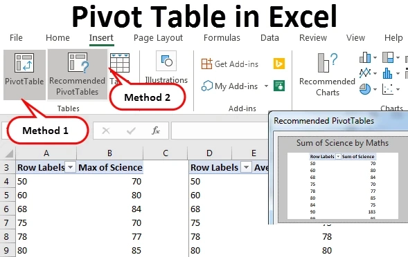
How to use
Let's get down to the nitty-gritty of building a pivot table now that you know what they're good for.
Enter your data into a range of rows and columns.
To create a pivot table in Excel, you must first create a standard Excel table in which to store your data. It's as simple as putting your data into a collection of rows and columns. You may classify your data using the topmost row or the topmost column.
Sorting your data.
Organizing your data so that it's simpler to work with in a pivot table begins with organizing the data you've already placed into your Excel sheet.
You may sort your data by clicking on the Sort icon just under the Data tab in your navigation bar at the top of the screen. You may sort your data by any column and in any order in the window that opens.
In order to sort your Excel spreadsheet by "Views to Date," pick this column title under Column and then choose whether you want to arrange your posts from smallest to biggest, or from largest to smallest.
Choose the cells you want to use as pivot points in your table.
Highlight the cells you want to summarize in a pivot table after you've inserted data into your Excel worksheet and sorted it according to your preferences. To insert a PivotTable, pick the PivotTable icon from the top menu. Select "PivotTable," then manually input the range of cells you want included in the PivotTable by clicking anywhere on your worksheet.
Optionally, you may choose whether or not to launch the pivot table in a new worksheet or maintain it inside the current one by selecting this option from the pop-up menu that appears. At the bottom of your Excel worksheet, a new sheet may be opened and closed. Then click OK to confirm your selection.
When you've finished creating your pivot table, you can begin adding fields to it.
If you're using a different version of Excel, your pivot table may seem somewhat different. As a rule, though, the fundamentals stay unchanged.
Using the "Values" section, add a new field by dragging and dropping it. Adding values to a field by dragging it into the Values box is the next step after deciding how to arrange your data.
For the sake of argument, let's assume you wish to describe the number of times a certain blog post has been seen by its title. The "Views" field would be dragged into the "Values" box.
Fine-tune your math.
It's possible to adjust the default calculation to anything like the average, maximum, or lowest, depending on what you're trying to find.
Value Field Settings may be found by clicking on the little upside-down triangle next to your value and selecting the option.