The XLOOKUP function in Excel is one of the most versatile tools for searching and retrieving data. While it’s straightforward to use XLOOKUP for single criteria, applying it to multiple criteria can significantly enhance its functionality, enabling you to handle complex datasets efficiently. In this guide, we will explore how to use XLOOKUP with multiple criteria step-by-step, complete with examples, tips, and best practices.

If you’ve been searching for terms like “XLOOKUP with multiple criteria” or “XLOOKUP multiple criteria,” this guide is tailored to provide all the insights you need.

What Is XLOOKUP?

XLOOKUP is a powerful Excel function that replaces older lookup functions like VLOOKUP, HLOOKUP, and INDEX-MATCH. Introduced in Excel 365 and Excel 2021, XLOOKUP allows you to:

• Search for a value in a range or array.
• Retrieve corresponding data from another range or array.
• Work seamlessly with exact or approximate matches.
• Search in both vertical and horizontal orientations.

Why Use XLOOKUP with Multiple Criteria?

While XLOOKUP is effective with single criteria, modern datasets often require searching based on multiple conditions. For instance, finding a sales record based on both product name and region requires combining multiple criteria.

Using XLOOKUP with multiple criteria allows you to:

• Handle more complex queries.
• Improve data accuracy.
• Streamline your data analysis workflows.

How to Use XLOOKUP with Multiple Criteria

Let’s dive into how you can set up XLOOKUP with multiple criteria. We’ll break this process into simple steps with examples.

Step 1: Understanding the Syntax of XLOOKUP

The basic syntax of XLOOKUP is:

=XLOOKUP(lookup_value, lookup_array, return_array, [if_not_found], [match_mode], [search_mode])

When working with multiple criteria, you modify the lookup_value and lookup_array to combine multiple conditions.

Step 2: Combine Criteria Using Helper Columns

A straightforward method for using XLOOKUP with multiple criteria is by combining the criteria into a helper column. Follow these steps:

1. Create a Helper Column:

• Concatenate the criteria columns into a single column.
• For example, if you want to combine “Product” and “Region,” use the formula:

=A2 & "," & B2

1. Apply XLOOKUP:

• Use the concatenated value as the lookup value.
• For example:

=XLOOKUP("Product1,Region1", HelperColumn, ReturnColumn)

Step 3: Use an Array Formula

If you prefer not to use helper columns, you can combine criteria directly within the XLOOKUP formula using an array. Here’s how:

1. Combine Criteria in the Lookup Value:

• Use an array constant or formula to represent multiple criteria.
• For example:

=XLOOKUP((A2=B2)*(C2=D2), LookupArray, ReturnArray)

1. Ensure Data Integrity:

• Make sure your criteria and return arrays align correctly.

Examples of XLOOKUP with Multiple Criteria

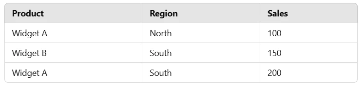
Example 1: Find Sales Data Based on Product and Region

Dataset:

Formula:

To find sales for “Widget A” in the “South” region:

=XLOOKUP("Widget A,South", HelperColumn, SalesColumn)

Example 2: Match Multiple Criteria Without a Helper Column

Dataset:

Formula:

To find John’s performance in IT:

=XLOOKUP((Employee="John")*(Department="IT"), PerformanceColumn)

Benefits of Using XLOOKUP Multiple Criteria

1. Greater Flexibility

Using multiple criteria enables more precise lookups tailored to your dataset’s complexity.

2. Enhanced Accuracy

By combining criteria, you reduce the risk of retrieving incorrect data due to duplicate entries.

3. Streamlined Workflows

Avoid creating additional lookup tables by leveraging the power of arrays or helper columns.

Limitations of XLOOKUP Multiple Criteria

While XLOOKUP is incredibly versatile, there are some limitations:

• Data Preparation: Using multiple criteria often requires well-structured datasets.
• Formula Complexity: Array formulas can become complex and challenging to debug.
• Performance Issues: For large datasets, complex XLOOKUP formulas can impact performance.

Tips and Best Practices for XLOOKUP Multiple Criteria

1. Use Named Ranges

Simplify your formulas by naming your ranges. For example:

=XLOOKUP(lookup_value, Products, Sales)

2. Test with Sample Data

Before applying the formula to large datasets, test it on a smaller subset to ensure accuracy.

3. Leverage Excel’s Evaluate Formula Tool

Use the “Evaluate Formula” feature to troubleshoot and understand how your XLOOKUP formula works.

4. Keep Arrays Consistent

Ensure that your lookup and return arrays are of the same size to avoid errors.

Alternatives to XLOOKUP for Multiple Criteria

If XLOOKUP doesn’t meet your needs, consider these alternatives:

INDEX-MATCH

Combine INDEX and MATCH with multiple criteria for flexible lookups. For example:

=INDEX(ReturnColumn, MATCH(1, (Criteria1=Column1)*(Criteria2=Column2), 0))

FILTER

The FILTER function is another excellent option for retrieving data based on multiple criteria. For example:

=FILTER(ReturnArray, (Criteria1=Column1)*(Criteria2=Column2))

Frequently Asked Questions About XLOOKUP Multiple Criteria

Can XLOOKUP Handle Multiple Criteria Directly?

Yes, XLOOKUP can handle multiple criteria by combining them into a single lookup value or using arrays.

Is XLOOKUP Better Than VLOOKUP for Multiple Criteria?

Yes, XLOOKUP is more flexible and eliminates the need for sorting or fixed column indexing, which are common limitations of VLOOKUP.

Can I Use XLOOKUP in Older Excel Versions?

No, XLOOKUP is only available in Excel 365 and Excel 2021. For older versions, consider using INDEX-MATCH or VLOOKUP.

Conclusion

Mastering XLOOKUP with multiple criteria can significantly enhance your Excel skills and productivity. Whether you’re managing sales data, employee performance, or complex datasets, XLOOKUP provides a robust solution for precise and efficient lookups.

By following the strategies and examples outlined in this guide, you’ll be well-equipped to handle advanced data retrieval tasks. Explore the power of XLOOKUP multiple criteria and unlock new possibilities in your Excel workflows!